Cauli-Det is a fine-tuned, architecturally modified YOLOv8 model that detects and localizes three cauliflower diseases from ordinary smartphone photos — 91.1% mAP, published in Frontiers in Plant Science (2024).

Code · Paper (DOI: 10.3389/fpls.2024.1373590)

Problem

Cauliflower is economically significant in agricultural economies like Bangladesh, which produced 283 kilotons in 2020 — but crop disease can devastate yield, and the standard defense is manual visual inspection, which is laborious, error-prone, and can miss early disease. Smallholder farmers, especially in remote areas, typically can’t afford expert agricultural consultation. Automated detection from an ordinary phone camera is the alternative — but it has to actually run on cheap hardware and actually tell you where the disease is, not just that the plant is sick.

That second point is the actual gap this project targets. Prior cauliflower-disease research — K-means clustering plus Random Forest, K-means plus GLCM features and logistic regression, transfer-learning approaches like EfficientNetB1 and InceptionV3 — is uniformly classification-only: “is this plant diseased, and with what,” not localization. For an actual field intervention (spot-treating, isolating one plant, flagging a specific area for closer inspection) you need to know where on the plant the disease is, which means object detection, not classification. That’s what motivates using YOLOv8 — a detector, not a classifier — as the base model.

Diseases covered

Three classes, drawn from field images collected in Manikganj, Bangladesh (Dec 2021 – Jan 2022):

• Downy Mildew (fungal) — white, yellow, or brownish patches with downy gray mold on leaf undersides, progressing to leaf death.
• Black Rot (bacterial, Xanthomonas campestris) — dull, irregular yellow spots progressing to V-shaped patches; renders produce unsaleable.
• Bacterial Spot Rot (Alternaria brassicicola) — water-soaked lesions on flower heads forming rotting masses, browning to black.

Architecture

Starting point: stock YOLOv8, which has three parts — a backbone (progressive downsampling convolutions extracting high-level features), a neck (C2f cross-stage-partial-fusion modules plus an SPPF spatial-pyramid-pooling module, fusing multi-scale features), and dual heads (detection, outputting bounding boxes; classification, outputting per-class probabilities).

Three deliberate, empirically-justified modifications on top of that:

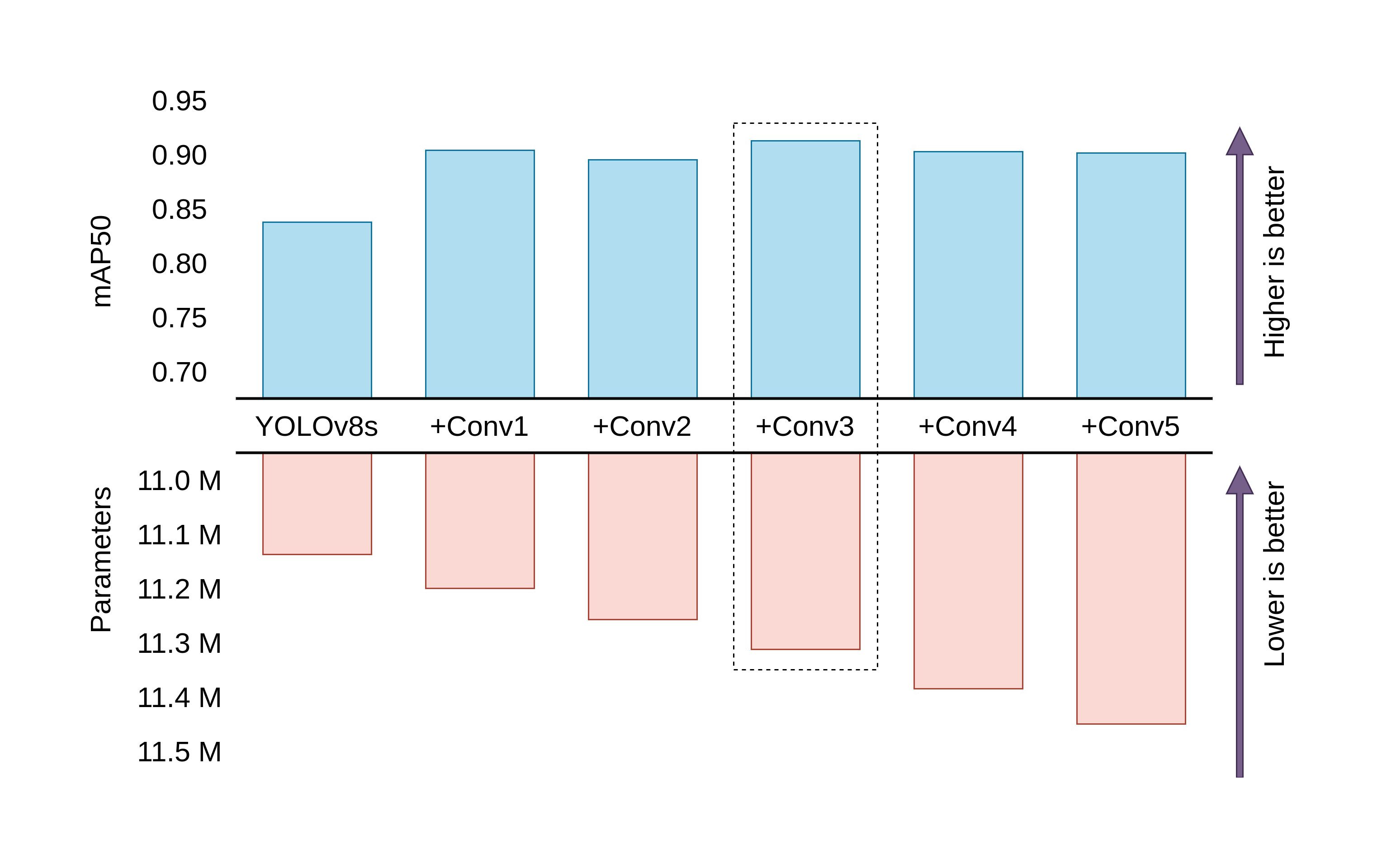
1. Extra Conv blocks in both heads (kernel size 1, inserted before the output convolution) — adds depth without much parameter growth. Landed on 3 extra blocks after testing 1 through 5.
2. Hard Swish activation, replacing the default SiLU — a clipped-linear approximation that trades a small amount of non-linearity for real compute savings, and happened to also win on accuracy.
3. Full (unfrozen) fine-tuning with a uniform learning rate across the whole network, rather than freezing the backbone or using differential learning rates. This was the single most consequential finding of the four ablations below.

Dataset

656 images total (VegNet dataset), split 70/15/15 train/val/test, resized to 256×256. Bounding boxes hand-annotated using Makesense.ai — the original dataset only had image-level labels, so this annotation work is itself part of the contribution.

Experiments — four questions, tested empirically

1. Which YOLO to start from?

YOLOv8s doesn’t win this table outright — YOLOv7 and YOLOv8m both post higher raw mAP. It was picked anyway on a deployability argument: under a third the parameters of YOLOv7, and the larger YOLOv8 variants show diminishing returns for a problem this size. The gap closes further once the head modifications below are applied.

2. How many extra Conv blocks?

+3 Conv blocks hits the best test mAP50 (90.6%) for near-minimal parameter cost; going further adds parameters without a corresponding gain — likely overfitting on a dataset this size.

3. Freeze the backbone, or fine-tune everything?

This is the sharpest result in the whole study. Freezing the backbone doesn’t just underperform — it collapses the model (mAP50 drops from 90.6% to as low as 27.2%). The pretrained COCO features aren’t close enough to cauliflower-field imagery for a frozen backbone to be a usable starting point; the domain shift is too large. Full fine-tuning was a necessity here, not a stylistic choice.

4. Which activation function?

Hard Swish wins on both axes that matter — best test mAP50 (91.1%) and cheaper to compute than SiLU — so it replaced the framework default.

Final results

Validation set — Precision 91.9%, Recall 85.1%, mAP50 92.0%, mAP50-95 67.7%

Test set — Precision 93.2%, Recall 82.6%, mAP50 91.1%, mAP50-95 70.1%

The weak point in both splits is Black Rot recall (66.7% on test) — the model catches Downy Mildew and Bacterial Spot Rot reliably but misses roughly a third of Black Rot instances. Worth naming explicitly rather than only quoting the headline mAP.

Honest limitations

1. Only three disease types — real cauliflower cultivation faces more than this; a dataset-scope limit, not a model-scope one.
2. No cross-device evaluation — all images from one camera; performance on typical farmer smartphone cameras is untested.
3. No real-time/field testing — evaluation is offline, on curated images; live video inference under field conditions hasn’t been tried.
4. Small dataset — 656 images total is small by detection-model standards, which limits generalization claims.

Full code, training scripts, and the complete README (including this same ablation detail) are on GitHub.

Sixteen reinforcement-learning agents independently scan small patches of a mammogram region of interest, communicate, and reach a consensus classification (benign/malignant) — without any single agent ever seeing the whole image. 82.45% accuracy on CBIS-DDSM. Published at IEEE ICDABI 2023, presented virtually.

Code · Paper (DOI: 10.1109/ICDABI60145.2023.10629500)

Problem

Breast carcinoma caused roughly 685,000 deaths in 2020 — 25% of that year’s 2.26 million new cases — and about 13% of women face a lifetime risk of developing it. Mammography is the standard screening tool, but reading mammograms is resource-intensive and requires expert radiologists, which is a bottleneck on early detection. Decades of computer-aided detection research have targeted this, but almost all of it — from classical ML through modern deep CNNs (state-of-the-art methods on CBIS-DDSM reach 95%+ accuracy) — processes the whole image at once. Parameter counts for these models scale with image resolution, an increasingly real cost as medical imaging resolution keeps climbing.

Reinforcement learning for this specific problem was, at the time, relatively unexplored. The question this project asks: what if, instead of one large model consuming the whole image, many small agents each look at a tiny local patch, share what they see with each other, and reach a decentralized consensus — does that reduce the computational burden of scaling with image size, while staying accurate enough to be useful? The architecture is adapted from prior multi-agent image classification work demonstrated on MNIST — this project’s contribution is extending that general framework to the harder, real task of mammogram ROI classification.

Architecture

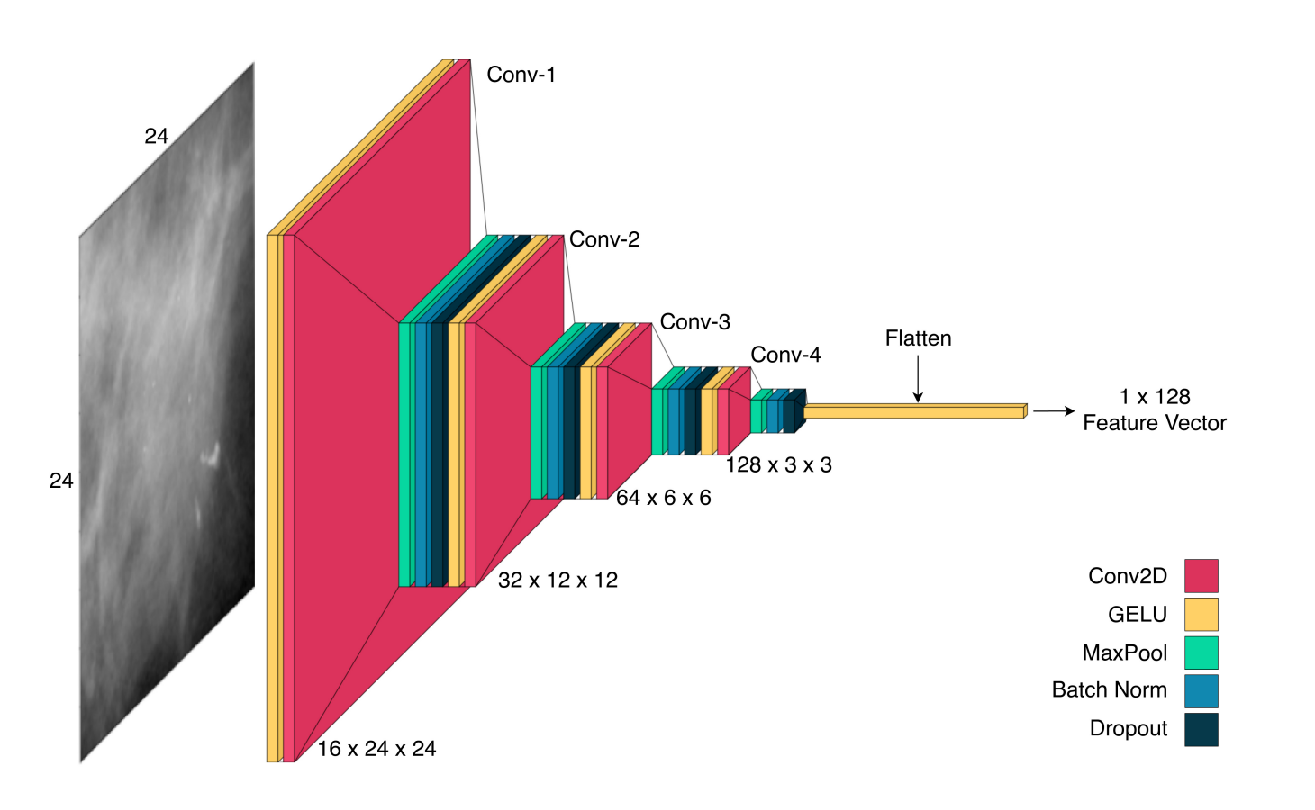
The task is framed as a partially observable Markov Decision Process (POMDP): an 8-tuple ⟨I, N, S, A, P, π, O, γ⟩ — the image, agent count, state space (agent positions), action space ({up, down, left, right}), position-transition function, action policy, local-observation function, and discount factor. Each of the 16 agents runs five modules per timestep:

1. Feature Extraction — a 4-layer CNN turns the agent’s local 24×24px window into a 128-dimensional feature vector.
2. Position Encoding — the agent’s (x, y) coordinates pass through a fully-connected layer, GELU activation, and batch normalization.
3. Decision — an LSTM aggregates the agent’s full observation history (its own features, position encoding, and the averaged messages received from other agents), then a small policy network outputs a probability distribution over the four move directions.
4. Prediction — a second, separate LSTM tracks a running benign/malignant belief from the same inputs, independent of the movement decision.
5. Communication — each agent generates a message from its prediction-LSTM hidden state, broadcasts it, and every other agent decodes and averages all incoming messages, feeding that average back into both LSTMs next timestep.

After a fixed episode length (32 steps by default), each agent emits a raw prediction vector; the system’s final classification is the argmax of the softmax-averaged predictions across all 16 agents. Training uses REINFORCE (policy-gradient) with an Adam optimizer — the reward for a sampled trajectory is the cross-entropy loss between that trajectory’s predicted and true label.

The key idea worth stating plainly: no agent ever sees the whole image, and there’s no central controller — classification emerges from many small, partial, locally-informed views reaching agreement through message-passing. That’s a genuinely different shape of solution than “bigger CNN, more parameters,” even though it doesn’t currently win on raw accuracy (see Results).

Dataset

CBIS-DDSM (Curated Breast Imaging Subset of DDSM), mass images only — calcification images were explicitly out of scope, left as future work. ROIs (professionally radiologist-annotated) resized to 224×224, retaining full aspect information.

Augmentation (horizontal flip, vertical flip, 90°/180°/270° rotation, and combinations) produced 12 copies per training image, expanding the training set to 15,816 images.

Training setup

100 epochs, mini-batch size 32, LSTM hidden size 256, message size 64, 16 agents with a 24×24px observation window, 32 steps per episode, discount factor γ=0.99, learning rate 1e-4, Adam optimizer.

Results

Comparison against other published methods on the same dataset (CBIS-DDSM, mass images):

The honest framing: this doesn’t beat CNN-based state of the art on raw accuracy — it lands in the middle of a six-method comparison table, behind four CNN-based methods and ahead of one. The paper’s own conclusion is blunt about this: the model is described as far from being useful in the field in its current form. The contribution being claimed is architectural and methodological — a decentralized, partial-observation approach that scales differently with image resolution than whole-image CNN classifiers — not a leaderboard win. That framing is worth keeping intact rather than softened; overstating a result like this is exactly what undermines credibility with a technical reviewer.

Honest limitations

1. Single dataset — evaluated only on CBIS-DDSM; generalization to other mammogram datasets untested.
2. Single abnormality type — trained only on mass images, not calcifications, which look visually distinct and would need separate evaluation.
3. Accuracy trails CNN competitors — see table above.
4. Requires pre-annotated ROIs — the system classifies a given ROI, it doesn’t locate the ROI on a raw, unmarked mammogram itself. Full automation would need an ROI-localization step on top of this.

Full code, training scripts, and the complete README are on GitHub.