
Cauli-Det, in Full: Problem, Architecture, and the Ablations Behind the 91.1% mAP
Published:
Cauli-Det is a fine-tuned, architecturally modified YOLOv8 model that detects and localizes three cauliflower diseases from ordinary smartphone photos — 91.1% mAP, published in Frontiers in Plant Science (2024).
Code · Paper (DOI: 10.3389/fpls.2024.1373590)
Problem
Cauliflower is economically significant in agricultural economies like Bangladesh, which produced 283 kilotons in 2020 — but crop disease can devastate yield, and the standard defense is manual visual inspection, which is laborious, error-prone, and can miss early disease. Smallholder farmers, especially in remote areas, typically can’t afford expert agricultural consultation. Automated detection from an ordinary phone camera is the alternative — but it has to actually run on cheap hardware and actually tell you where the disease is, not just that the plant is sick.
That second point is the actual gap this project targets. Prior cauliflower-disease research — K-means clustering plus Random Forest, K-means plus GLCM features and logistic regression, transfer-learning approaches like EfficientNetB1 and InceptionV3 — is uniformly classification-only: “is this plant diseased, and with what,” not localization. For an actual field intervention (spot-treating, isolating one plant, flagging a specific area for closer inspection) you need to know where on the plant the disease is, which means object detection, not classification. That’s what motivates using YOLOv8 — a detector, not a classifier — as the base model.
Diseases covered
Three classes, drawn from field images collected in Manikganj, Bangladesh (Dec 2021 – Jan 2022):
- Downy Mildew (fungal) — white, yellow, or brownish patches with downy gray mold on leaf undersides, progressing to leaf death.
- Black Rot (bacterial, Xanthomonas campestris) — dull, irregular yellow spots progressing to V-shaped patches; renders produce unsaleable.
- Bacterial Spot Rot (Alternaria brassicicola) — water-soaked lesions on flower heads forming rotting masses, browning to black.
Architecture
Starting point: stock YOLOv8, which has three parts — a backbone (progressive downsampling convolutions extracting high-level features), a neck (C2f cross-stage-partial-fusion modules plus an SPPF spatial-pyramid-pooling module, fusing multi-scale features), and dual heads (detection, outputting bounding boxes; classification, outputting per-class probabilities).
Three deliberate, empirically-justified modifications on top of that:
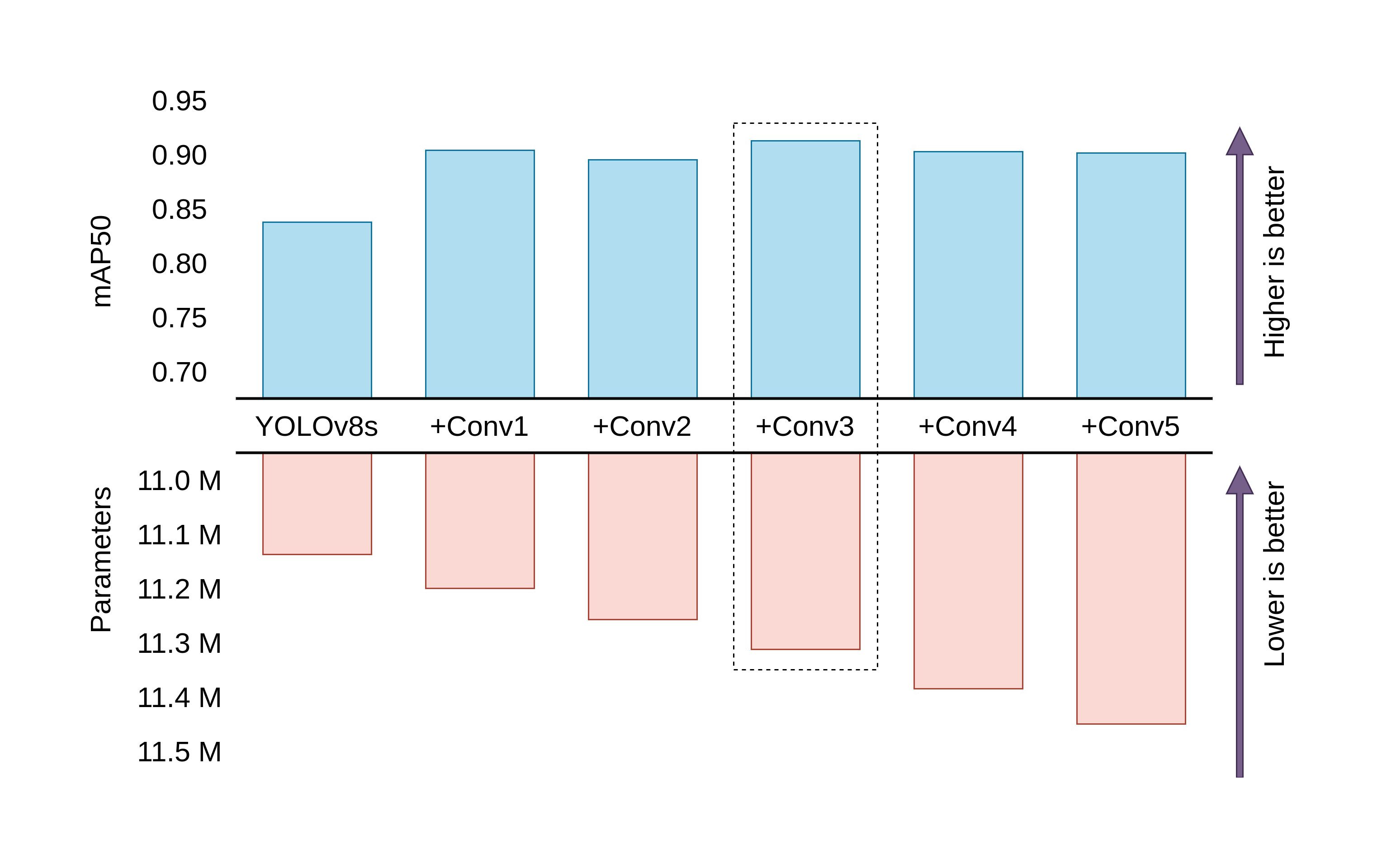
- Extra Conv blocks in both heads (kernel size 1, inserted before the output convolution) — adds depth without much parameter growth. Landed on 3 extra blocks after testing 1 through 5.
- Hard Swish activation, replacing the default SiLU — a clipped-linear approximation that trades a small amount of non-linearity for real compute savings, and happened to also win on accuracy.
- Full (unfrozen) fine-tuning with a uniform learning rate across the whole network, rather than freezing the backbone or using differential learning rates. This was the single most consequential finding of the four ablations below.
Dataset
656 images total (VegNet dataset), split 70/15/15 train/val/test, resized to 256×256. Bounding boxes hand-annotated using Makesense.ai — the original dataset only had image-level labels, so this annotation work is itself part of the contribution.
| Class | Share | Train | Val | Test | Total |
|---|---|---|---|---|---|
| Healthy | 31.4% | 144 | 31 | 31 | 206 |
| Downy Mildew | 27.0% | 125 | 26 | 26 | 177 |
| Bacterial Spot Rot | 26.4% | 121 | 26 | 26 | 173 |
| Black Rot | 15.2% | 70 | 15 | 15 | 100 |
Experiments — four questions, tested empirically
1. Which YOLO to start from?
| Model | Test Precision | Test Recall | Test mAP50 | Test mAP50-95 | Params |
|---|---|---|---|---|---|
| YOLOv7 | 97.8% | 88.9% | 92.6% | 71.8% | 37.21M |
| YOLOv8n | 91.0% | 82.8% | 82.1% | 57.7% | 3.01M |
| YOLOv8s | 91.4% | 83.2% | 84.1% | 66.1% | 11.14M |
| YOLOv8m | 91.2% | 86.8% | 91.6% | 72.1% | 25.86M |
| YOLOv8l | 90.4% | 87.5% | 91.5% | 71.1% | 43.63M |
| YOLOv8x | 91.8% | 84.7% | 91.0% | 72.3% | 68.16M |
YOLOv8s doesn’t win this table outright — YOLOv7 and YOLOv8m both post higher raw mAP. It was picked anyway on a deployability argument: under a third the parameters of YOLOv7, and the larger YOLOv8 variants show diminishing returns for a problem this size. The gap closes further once the head modifications below are applied.
2. How many extra Conv blocks?
| Config | Test Precision | Test Recall | Test mAP50 | Test mAP50-95 | Params |
|---|---|---|---|---|---|
| YOLOv8s (base) | 91.4% | 83.2% | 84.1% | 66.1% | 11.14M |
| +1 Conv | 95.5% | 83.7% | 90.5% | 68.8% | 11.20M |
| +2 Conv | 90.1% | 85.2% | 89.4% | 69.4% | 11.26M |
| +3 Conv | 93.1% | 82.9% | 90.6% | 69.4% | 11.32M |
| +4 Conv | 93.6% | 85.9% | 90.3% | 68.6% | 11.38M |
| +5 Conv | 94.6% | 85.7% | 90.4% | 68.8% | 11.45M |
+3 Conv blocks hits the best test mAP50 (90.6%) for near-minimal parameter cost; going further adds parameters without a corresponding gain — likely overfitting on a dataset this size.
3. Freeze the backbone, or fine-tune everything?
| Strategy | Test Precision | Test Recall | Test mAP50 | Test mAP50-95 |
|---|---|---|---|---|
| Default (uniform, unfrozen) | 93.1% | 82.9% | 90.6% | 69.4% |
| Freeze non-extra-Conv layers | 29.9% | 35.2% | 27.2% | 13.6% |
| Freeze backbone | 56.6% | 46.1% | 51.1% | 28.0% |
| Fast extra-Conv (differential LR) | 90.6% | 76.5% | 83.9% | 60.3% |
| Fast head (differential LR) | 92.0% | 77.8% | 84.6% | 61.5% |
| Fast head+neck (differential LR) | 95.5% | 83.7% | 90.5% | 68.8% |
This is the sharpest result in the whole study. Freezing the backbone doesn’t just underperform — it collapses the model (mAP50 drops from 90.6% to as low as 27.2%). The pretrained COCO features aren’t close enough to cauliflower-field imagery for a frozen backbone to be a usable starting point; the domain shift is too large. Full fine-tuning was a necessity here, not a stylistic choice.
4. Which activation function?
| Function | Test Precision | Test Recall | Test mAP50 | Test mAP50-95 |
|---|---|---|---|---|
| SiLU (default) | 93.1% | 82.9% | 90.6% | 69.4% |
| ReLU | 90.6% | 82.9% | 87.5% | 66.8% |
| LeakyReLU | 94.2% | 84.0% | 90.0% | 67.7% |
| Tanh | 90.6% | 70.2% | 77.1% | 50.2% |
| Hard Swish | 93.2% | 82.6% | 91.1% | 70.1% |
Hard Swish wins on both axes that matter — best test mAP50 (91.1%) and cheaper to compute than SiLU — so it replaced the framework default.
Final results
Validation set — Precision 91.9%, Recall 85.1%, mAP50 92.0%, mAP50-95 67.7%
| Class | Images | Instances | Precision | Recall | AP50 | AP50-95 |
|---|---|---|---|---|---|---|
| Downy Mildew | 26 | 77 | 91.9% | 84.4% | 94.1% | 70.3% |
| Black Rot | 15 | 215 | 85.2% | 75.8% | 84.5% | 53.2% |
| Bacterial Spot Rot | 26 | 40 | 98.7% | 95.0% | 97.4% | 79.7% |
Test set — Precision 93.2%, Recall 82.6%, mAP50 91.1%, mAP50-95 70.1%
| Class | Images | Instances | Precision | Recall | AP50 | AP50-95 |
|---|---|---|---|---|---|---|
| Downy Mildew | 26 | 50 | 90.1% | 84.0% | 92.5% | 68.6% |
| Black Rot | 15 | 225 | 92.6% | 66.7% | 82.6% | 55.2% |
| Bacterial Spot Rot | 26 | 34 | 96.8% | 97.1% | 98.3% | 86.4% |
The weak point in both splits is Black Rot recall (66.7% on test) — the model catches Downy Mildew and Bacterial Spot Rot reliably but misses roughly a third of Black Rot instances. Worth naming explicitly rather than only quoting the headline mAP.
Honest limitations
- Only three disease types — real cauliflower cultivation faces more than this; a dataset-scope limit, not a model-scope one.
- No cross-device evaluation — all images from one camera; performance on typical farmer smartphone cameras is untested.
- No real-time/field testing — evaluation is offline, on curated images; live video inference under field conditions hasn’t been tried.
- Small dataset — 656 images total is small by detection-model standards, which limits generalization claims.
Full code, training scripts, and the complete README (including this same ablation detail) are on GitHub.